
Artificial Intelligence has been witnessing a monumental growth in bridging the gap between the capabilities of humans and machines. One of the coolest thing that I have worked on was Image Recognition, that combines Computer Vision and Deep Neural Networks. The advancements in Computer Vision with Deep Learning has been constructed and perfected with time, primarily over one particular algorithm – a Convolutional Neural Network which is fundamentally used in Image Recognition.
In this blog, I will show you 2 ways on creating your own Image Classifier model – a code that will be able to identify or classify objects in a picture.
The first way which I call it the “Daredevil approach” and the second way which I call it the “Hacker style”.
Before getting our hands Dirty, I adamantly believe that Learning from scratch will help us to have a firm understanding on a higher level.
By the way, I will make sure that there is minimal math involved while explaining the concept.
My sarcastic Apologies…
![]()
Let’s start
Contents
Image Recognition
Convolutional Neural Network:
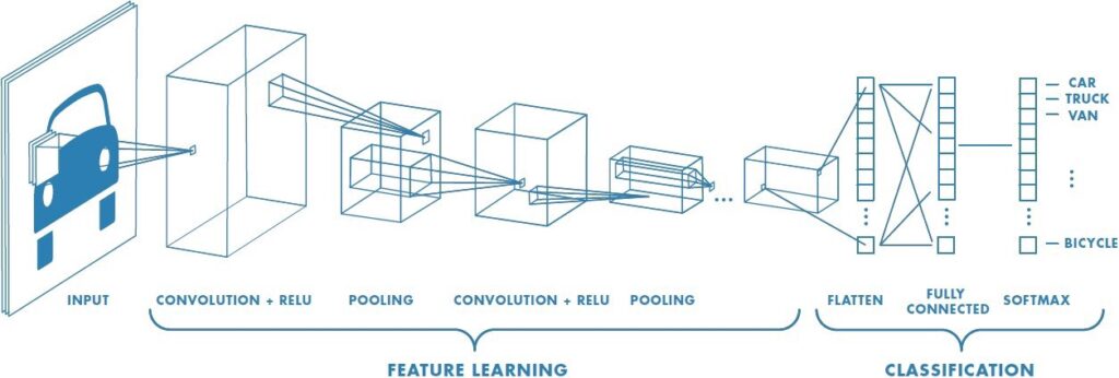
A Convolutional Neural Network (ConvNet/CNN) is a Deep Learning algorithm which can take in an input image, assign importance (learnable weights and biases) to various aspects/objects in the image and be able to differentiate one from the other. The pre-processing required in a ConvNet is much lower as compared to other classification algorithms.
The architecture of a ConvNet is analogous to that of the connectivity pattern of Neurons in the Human Brain and was inspired by the organization of the Visual Cortex. Individual neurons respond to stimuli only in a restricted region of the visual field known as the Receptive Field. A collection of such fields overlap to cover the entire visual area.
On a higher level, the layers of a CNN consist of an input layer, an output layer and a hidden layer that includes multiple convolutional layers, pooling layers, fully connected layers, and normalization layers.
 Information that should know before getting into CNN
What is a Picture or Image…?
At a Higher Level, a picture can be represented with the help of a pixel. Each pixel has 3 major color band- usually called the RGB Color. In addition to this, each pixel also has a fourth parameter called the Alpha parameter.
Alpha is a measure of how opaque an image is. The higher the number, the more solid the color is, the lower the number, the more transparent it is.
So each pixel is measured in RGBA, example row is [255, 255, 255, 255], which means we’re looking at a 256-color image since programming starts with a 0 rather than a 1. This color means 255 red, 255 green, 255 blue, and then 255 Alpha.
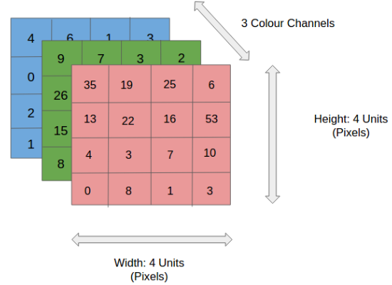
![]() For simplicity sake, let’s forget the Alpha parameter. In the below figure, we have an RGB image which has been separated by its three color channels— Red, Green, and Blue. There are a number of such color spaces in which images exist — Grayscale, RGB, HSV, CMYK, etc.
For simplicity sake, let’s forget the Alpha parameter. In the below figure, we have an RGB image which has been separated by its three color channels— Red, Green, and Blue. There are a number of such color spaces in which images exist — Grayscale, RGB, HSV, CMYK, etc.
 Convolution Operation…
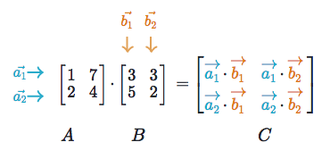
To be honest, this is where the fun starts. CNN gets its name because of this operation. On a higher level, Convolution Operation is nothing but “Dot Product ” of 2 matrices. One matrix is the input Image whereas the second matrix is what we called the “Convolution filter” or “Kernel”.The main point of this operation is the ability to generate Feature map.
Convolution Filter or Kernel….?
In image processing, a kernel, convolution matrix is a small matrix. It is used for blurring, sharpening, embossing, edge detection, and more. This is accomplished by doing a convolution between a kernel and an image.
 Commonly used filters:
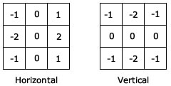 The Sobel filter
Instead of using these filters, we can create our own as well and treat them as a parameter which the model will learn using backpropagation.
Padding….?
Every time we apply a convolutional operation, the size of the image shrinks. Pixels present in the corner of the image are used only a few numbers of times during convolution as compared to the central pixels. Hence, we do not focus too much on the corners since that can lead to information loss.
To overcome these issues, we can pad the image with an additional border, i.e., we add one pixel all around the edges. This means that the input will be an 8 X 8 matrix if the input image has a dimension of a 6 X 6 matrix. Applying convolution of 3 X 3 on it will result in a 6 X 6 matrix which is the original shape of the image.
This raises the question “How do you know the result is gonna be 6×6″…?
Let me explain…..
Its obvious… simple math… Come on
or
Mathematically:
(n+2p-f+1) X (n+2p-f+1)

where,

n - Input Image dimension

p - padding size

f - filter dimension
There are two common choices for padding:
Valid:
It means no padding. If we are using valid padding, the output will be (n-f+1) X (n-f+1)
Same: Here, we apply padding so that the output size is the same as the input size,
i.e.,

n+2p-f+1 = n

So, p = (f-1)/2
Stride…?
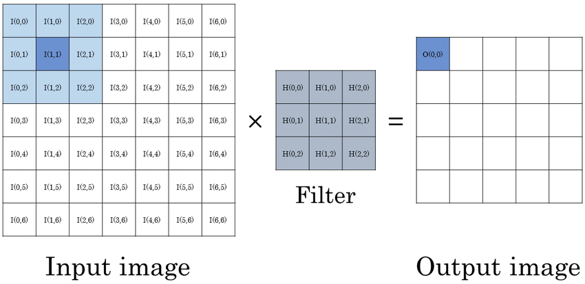
Stride is the number of pixels shifts over the input matrix. When the stride is 1 then we move the filters to 1 pixel at a time. When the stride is 2 then we move the filters to 2 pixels at a time and so on. The below figure shows convolution would work with a stride of 1.
 So, if u want to know the output after stride has been applied:
Mathematically:
[(n+2p-f)/s+1] X [(n+2p-f)/s+1]

where,

n - Input Image dimension

p - padding size

f - filter dimension

s - stride
Example Convolution Process
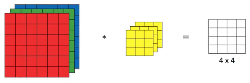
Concerning simplicity’s sake, let’s consider an image of dimension 6x6x3 with a kernel 3x3x3 with a stride of 1.
Input: 6 X 6 X 3
Filter: 3 X 3 X 3
Stride: 1
NOTE: Keep in mind that the number of channels in the input and filter should be the same.
This will result in an output of 4 X 4. Let’s understand it visually:
 Let’s say, instead of using just a single filter, we can use multiple filters. Let’s assume the first filter will detect vertical edges and the second filter will detect horizontal edges from the image. So, instead of having a 4 X 4 output as in the above example, we would have a 4 X 4 X 2 output where 2 is the number of filters used.
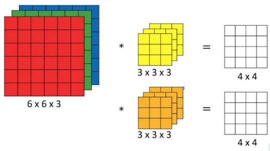 So, Mathematically,
[(n+2p-f)/s+1] X [(n+2p-f)/s+1] X n'

where,

n - Input Image dimension

p - padding size

f - filter dimension

s - stride

n' - number of filter used
Pooling Operation:
A pooling layer is another building block of a CNN. Pooling operation is generally used to reduce the size of the inputs and hence speed up the computation. Pooling layer operates on each feature map independently.
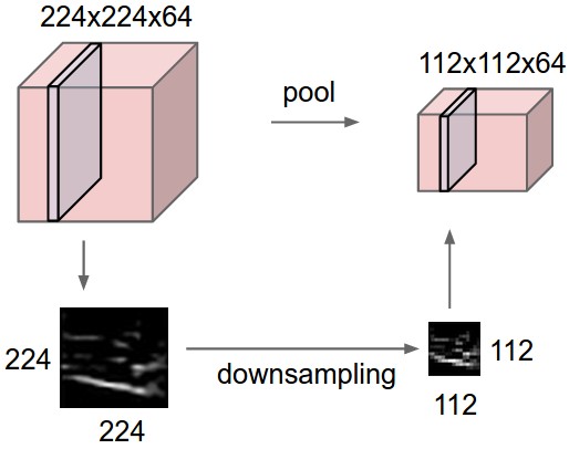 The most common approach used in pooling is max pooling.
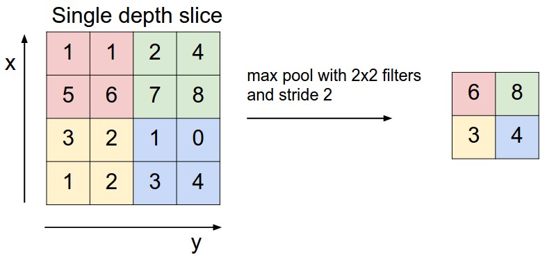 For every consecutive 2 X 2 block, we take the max number.
Here, we have applied a filter of size 2 and a stride of 2. These are the hyperparameters for the pooling layer. Apart from max pooling, we can also apply average pooling where, instead of taking the max of the numbers, we take their average.
To sum up, the hyperparameters for a pooling layer are:
- Filter size
- Stride
- Max or average pooling
Mathematically:
If the input of the pooling layer is

nh X nw X nc,

then the output will be,

[{(nh – f) / s + 1} X {(nw – f) / s + 1} X nc].

where,

nh - height

nw - width

nc - number of chanell

f - filter dimension

s - stride
I know this is a little too much… but I think is more than enough for anyone to understand how image recognition works.
In my next blog, we will have a look at how to build a deep neural network with the concept that we just learned.