First of all, we’re super excited to show you how to solve any Sudoku puzzle in less than a second. At the end of this article, we’re pretty sure that you will be leaving with a solid perception of concepts like “Constraint Propagation” and a popular Search Algorithm “Depth First Search”.
This blog is inspired by Peter Norvig, Director of Research Google, and one of his recent articles. I definitely recommend you to read his blog.
Before getting our hands messy, let’s get to know the game and some terminologies that we will be using.
Contents
SUDOKU:
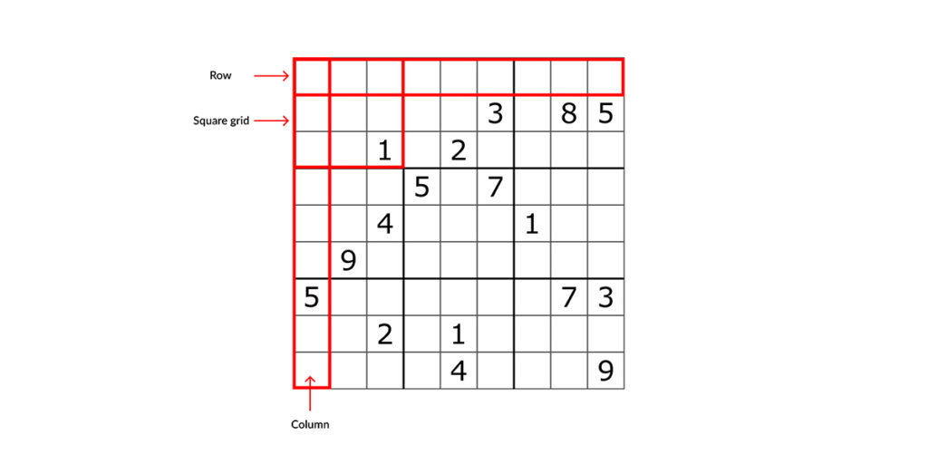
“Sudoku is a logic-based, combinatorial number-placement puzzle. The aim is to fill a 9×9 grid with digits, so that each column, each row, and each of the nine 3×3 sub-grids that compose the grid (also called “boxes,” “blocks,” or “regions”) contain all of the digits from 1 to 9. The puzzle setter provides a partially completed grid, which for a well-posed puzzle has a single solution.” – Wikipedia
GRID: Each individual square in Sudoku. So, there are 81 grids in any Sudoku Puzzle.
ROWS: Each row in Sudoku.
COLUMNS: Each column in Sudoku.
UNIT: Each Unit has 9 squares (column, row, or box) in it.
SQUARE UNIT: Each sub-box within a Sudoku Puzzle. So, a complete Sudoku puzzle is composed of 9 square units.
PEERS: Squares that share a unit.


We know, that’s a lot of information to process. Bare with us, once you can get ahold of this, half of the problem will be over.
Another major part of this is understanding “Constraint Propagation” and “Depth First Search”.
FUN PART:
Let’s start implementing the things that we just read now.
We know for a fact that a 9×9 Sudoku puzzle will have 9 rows and 9 columns.
Let’s consider:
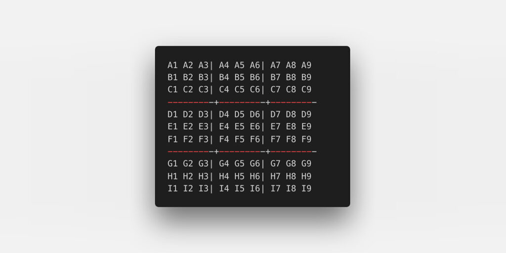
Rows ranging from A, B, C to Letter I (for a total of 9 letters).
Columns ranging from 1,2,3 to number 9 (for a total of 9 numbers, and to avoid confusion).
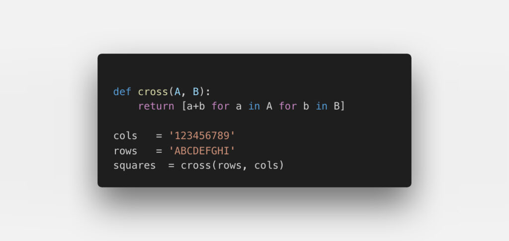
This implies that each grid in the puzzle will have a name for reference, and whose name will range from A1, A2 to I8, I9.
 CODE:
CODE:
 The next step is to find all the rows, columns, and squares, and Python makes it simple in achieving this task.
CODE:
 The next step is to find all the peers with respect to a grid.
CODE:
 This marks the end of this article, because we feel like this a little too much for a single day and the concept of “Constraint Propagation” deserves its very own blog. We will explain this with other examples so that it will be easier to understand.


